
Notice
Recent Posts
Recent Comments
Link
| 일 | 월 | 화 | 수 | 목 | 금 | 토 |
|---|---|---|---|---|---|---|
| 1 | 2 | 3 | 4 | 5 | ||
| 6 | 7 | 8 | 9 | 10 | 11 | 12 |
| 13 | 14 | 15 | 16 | 17 | 18 | 19 |
| 20 | 21 | 22 | 23 | 24 | 25 | 26 |
| 27 | 28 | 29 | 30 |
Tags
- python 갯수세기
- 카카오
- 에러해결
- Pycaret
- RMES
- 스택
- 평가지표
- PAPER
- knn
- mes
- 프로그래머스
- Mae
- Alignments
- TypeError
- MAPE
- iNT
- Overleaf
- Tire
- 논문작성
- KAKAO
- mMAPE
- Python
- 파이썬을파이썬답게
- 코테
- 논문
- SMAPE
- n_neighbors
- n_sample
- Scienceplots
- 논문editor
Archives
- Today
- Total
EunGyeongKim
그래프 그리기 본문
ref:파이썬으로 배우는 머신러닝의 교과서
2차원 그래프 그리기
그래프를 그리기 위해 matplotlib의 pyplot라이브러리를 import 하고 plt라는 별칭을 만들어 사용.
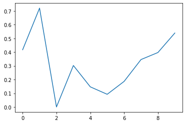
임의의 그래프 그리기
import numpy as np
import matplotlib.pyplot as plt
%matplotlib inline

#data
np.random.seed(1) # fix random seed
x = np.arange(10)
y = np.random.rand(10)

#graph
plt.plot(x, y)
plt.show()
프로그램 리스트 규칙
리스트 번호 1-(1), 1-(2), 1-(3), 2-(1)과 같음
괄호 앞의 숫자가 같은 리스트는 변수를 공유하는 리스트, 괄호 안의 숫자 순서대로 실행한다고 가정함.
1-(1)에서 만든 변수와 함수는 1-(2), 1-(3)에서 사용가능함.
지금까지의 이력을 메모리에서 삭제할 때
%reset%reset 명령어 입력
3차원 그래프 그리기
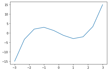
f(x) = (x-2)x(x+2) 그래프 그리기
import numpy as np
import matplotlib.pyplot as plt
%matplotlib inline

#define f(x)
def f(x):
    return (x-2) * x * (x+2)

# check f(x)
print(f(np.array([1,2,3])))
# [-3  0 15]

# set x value (method 1)
x = np.arange(-3, 3.5, 0.5)
print(x)
# [-3.  -2.5 -2.  -1.5 -1.  -0.5  0.   0.5  1.   1.5  2.   2.5  3. ]

# set x value (method 2)
x = np.linspace(-3, 3, 10) # -3 ~ 3, len(x) = 10
print(np.round(x, 2))
# [-3.   -2.33 -1.67 -1.   -0.33  0.33  1.    1.67  2.33  3.  ]

# graph
plt.plot(x, f(x))
plt.show()
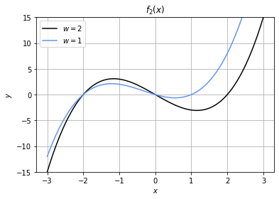
그래프 장식하기
import numpy as np
import matplotlib.pyplot as plt
%matplotlib inline

#define f(x)
def f2(x, w):
    return (x-2) * x * (x+2)

# define x value
x = np.linspace(-3, 3, 100)

#chart
plt.plot(x, f2(x, 2), color='black', label = '$w=2$')
plt.plot(x, f2(x, 1), color='cornflowerblue', label = '$w=1$')
plt.legend(loc="upper left")
plt.ylim(-15, 15) # range of y
plt.title('$f_2(x)$')
plt.xlabel('$x$')
plt.ylabel('$y$')
plt.grid(True) # grid
plt.show()
사용할 수 있는 색상 목록
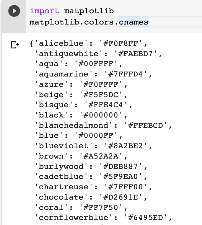
import matplotlib
matplotlib.colors.cnames
그래프 여러개 보여주기(plt.subplot(n1, n2, n))
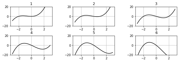
plt.figure(figsize=(10, 3))
plt.subplots_adjust(wspace = 0.5, hspace=0.5) #그래프 간격 지정
for i in range(6):
    plt.subplot(2, 3, i+1) #그래프 위치
    plt.title(i+1)
    plt.plot(x, f2(x, i), 'k')
    plt.ylim(-20, 20)
    plt.grid(True)
plt.show()
3차원 그래프 그리기
3차원 그래프 그리기
$$f(x_0, x_1) = (2x^2_0 + x^2_1)exp(-(2x^2_0+x^2_1)) 그래프 그리기$$
위 식을 계산하는 함수 만들기
import numpy as np
import matplotlib.pyplot as plt

# define f3
def f3(x0, x1):
    r = 2 * x0 ** 2 + x1 **2
    ans = r * np.exp(-r)
    return ans

# cal f3
xn = 9
x0 = np.linspace(-2, 2, xn)
x1 = np.linspace(-2, 2, xn)
y = np.zeros((len(x0), len(x1)))
for i0 in range(xn):
    for i1 in range(xn):
        y[i1, i0] = f3(x0[i0], x1[i1])

print(x0)
#[-2.  -1.5 -1.  -0.5  0.   0.5  1.   1.5  2. ]

print(np.round(y, 1))
#[[0.  0.  0.  0.  0.1 0.  0.  0.  0. ]
# [0.  0.  0.1 0.2 0.2 0.2 0.1 0.  0. ]
# [0.  0.  0.1 0.3 0.4 0.3 0.1 0.  0. ]
# [0.  0.  0.2 0.4 0.2 0.4 0.2 0.  0. ]
# [0.  0.  0.3 0.3 0.  0.3 0.3 0.  0. ]
# [0.  0.  0.2 0.4 0.2 0.4 0.2 0.  0. ]
# [0.  0.  0.1 0.3 0.4 0.3 0.1 0.  0. ]
# [0.  0.  0.1 0.2 0.2 0.2 0.1 0.  0. ]
# [0.  0.  0.  0.  0.1 0.  0.  0.  0. ]]
계산한 수치를 색으로 표현하기 : pcolor
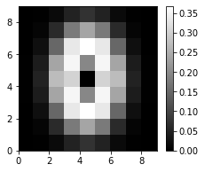
plt.figure(figsize=(3.5, 3))
plt.gray()
plt.pcolor(y)
plt.colorbar()
plt.show()
계산한 함수의 표면을 표시 : surface

from mpl_toolkits.mplot3d import Axes3D

xx0, xx1 = np.meshgrid(x0, x1)

plt.figure(figsize=(5, 3.5))
ax = plt.subplot(1,1,1, projection='3d')
ax.plot_surface(xx0, xx1, y, rstride = 1, cstride = 1, alpha = 0.3,
                color = 'blue', edgecolor = 'black')
ax.set_zticks((0, 0.2))
ax.view_init(75, -95)
plt.show()
계산한 함수의 표면을 표시(2) : surface

from mpl_toolkits.mplot3d import Axes3D

xx0, xx1 = np.meshgrid(x0, x1)

plt.figure(figsize=(5, 3.5))
ax = plt.subplot(1,1,1, projection='3d')
ax.plot_surface(xx0, xx1, y, rstride = 1, cstride = 1, alpha = 0.3,
                color = 'blue', edgecolor = 'black')
ax.set_zticks((0, 0.2))
ax.view_init(0, -95)
plt.show()
등고선으로 표시 : contour
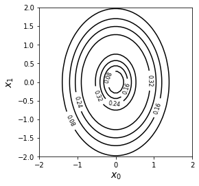
xn = 50
x0 = np.linspace(-2, 2, xn)
x1 = np.linspace(-2, 2, xn)

y = np.zeros((len(x0), len(x1)))
for i0 in range(xn):
    for i1 in range(xn):
        y[i1, i0] = f3(x0[i0], x1[i1])

xx0, xx1 = np.meshgrid(x0, x1)

plt.figure(figsize=(4,4))
cont = plt.contour(xx0, xx1, y, 5, colors='black') # 5 <-등고선 개수
cont.clabel(fmt = '%3.2f', fontsize=8)
plt.xlabel('$x_0$', fontsize =14)
plt.ylabel('$x_1$', fontsize =14)
plt.show()
'ML & DL' 카테고리의 다른 글
| 미분, 편미분 (0) | 2023.02.20 |
|---|---|
| 머신러닝에 필요한 수학과 numpy코드 (0) | 2023.02.20 |
| [데이터 전처리] 정규화 (Normalization) (0) | 2022.08.11 |
| 딥러닝 단어 정리 (0) | 2022.07.23 |
| [NN] MNIST 분류 Neural Network (0) | 2022.07.22 |
'ML & DL' Related Articles
more
Comments