
| 일 | 월 | 화 | 수 | 목 | 금 | 토 |
|---|---|---|---|---|---|---|
| 1 | 2 | 3 | 4 | 5 | ||
| 6 | 7 | 8 | 9 | 10 | 11 | 12 |
| 13 | 14 | 15 | 16 | 17 | 18 | 19 |
| 20 | 21 | 22 | 23 | 24 | 25 | 26 |
| 27 | 28 | 29 | 30 |
- n_neighbors
- 코테
- Alignments
- 프로그래머스
- Mae
- n_sample
- PAPER
- TypeError
- iNT
- Overleaf
- Python
- 파이썬을파이썬답게
- MAPE
- 논문작성
- 평가지표
- 에러해결
- Scienceplots
- Tire
- mMAPE
- python 갯수세기
- mes
- 논문
- 논문editor
- KAKAO
- 카카오
- RMES
- 스택
- Pycaret
- SMAPE
- knn
- Today
- Total
EunGyeongKim
가우스 함수(Gaussian Function) 본문
가우스 함수는 x=0을 중심으로 종 모양을 하고 있다. 가우스 함수는 곡선을 근사하는 기저함수로 사용된다.
가우스 함수의 식의 기본형 식
$$y = exp(-x^2)$$
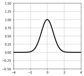
import numpy as np
import matplotlib.pyplot as plt
%matplotlib inline

def gauss(mu, sigma, a):
    return a*np.exp(-(x-mu)**2 / sigma **2)

x = np.linspace(-4, 4, 100)
plt.figure(figsize=(4,4))
plt.plot(x, gauss(0,1,1), 'black', linewidth=3)
plt.ylim(-.5, 1.5)
plt.xlim(-4,4)
plt.grid(True)
plt.show()
함수의 중심을 μ, 확산되는 크기(표준편차)를 σ, 높이를 a로 하여 조절 가능한 형태로 수정한 식
$$y = a*exp(-\frac{(x-\mu)^2}{\sigma^2})$$
가우스 함수의 확률분포
가우스 함수의 확률분포를 구할 경우에는 x에 관한 적분이 1이 되도록 식
$$a = \frac{1}{(2\pi \sigma^2)^{1/2}}$$
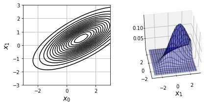
2차원 가우스 함수
가우스 함수에서 사용하는 입력을 2차원 벡터인 x=[x0, x1]^T 라고 했을때 가우스 함수의 기본형
$$y = exp\left\{ - (x_0^2 + x^2_1) \right\}$$
이 기본형을 중심을 이동시키거나 길게 만들기 위해 몇가지 매개변수를 더한 형태의 식
$$y = a\cdot exp\left\{-\frac{1}{2}(x-\mu)^T\sum ^{-1}(x-\mu) \right\}$$
함수의 형태를 나타내는 매개변수(μ : 평균벡터(중심벡터). 분포의 중심을 나타냄 , ∑ : 공분산행렬.)
여기서 ∑는 공분산 행렬로, 2*2행렬입니다.
$$\sum = \begin{bmatrix}\sigma_0 & \sigma_2 \\\sigma_2 & \sigma_1 \\\end{bmatrix}$$
σ0, σ1 : x0의 방향과 x1방향의 분포의 퍼짐을 나타냄
σ2 : 분포의 기울기 (x0, x1의 상관관계)에 대응. 양수하면 오른쪽을 치우친 분포, 음수이면 왼쪽으로 치우친 분포
exp()안에는 벡터나 행렬이 들어가 있음 (=스칼라 양)
μ =[μ0, μ1]^T라고 했을 때 (x-μ)^T(x-μ)계산
$$(x-\mu)^T\sum^{-1}(x-\mu) = x^T\sum^{-1}x$$
$$=[x_0, x_1]\cdot\frac{1}{\sigma_0\sigma_1-\sigma_2^2}\begin{bmatrix}\sigma_1 & -\sigma_2 \\
-\sigma_2 & \sigma_0 \\\end{bmatrix}\begin{bmatrix}x_0 \\x_1\end{bmatrix} $$
$$ = \frac{1}{\sigma_0\sigma_1 - \sigma_2^2}(\sigma_1x_0^2 - 2\sigma_2x_0x_1 + \sigma_0x_1^2)$$
exp의 내용의 실체는 x0와 x1의 2차식임을 알 수 있음
a는 가우스 함우에서 확률분포를 나타내는 경우 다음과 같이 설정
$$a = \frac{1}{2\pi}\frac{1}{|\sum|^{1/2}}$$
위처럼 하면 입력공간에서의 적분값이 1이고, 함수가 확률분포를 표현할 수 있음.
|∑|는 행렬식으로 불리는 양. 2*2 행렬인경우 다음 공식으로 계산된 양임
$$\left| A\right| = \begin{vmatrix}a & b \\c & d \\\end{vmatrix} = ad-cb$$
따라서 |∑|는 다음과 같이 나타낼 수 있음
$$\left| \sum \right| =\sigma_0\sigma_1 - \sigma_2^2$$
import numpy as np
import matplotlib.pyplot as plt
from mpl_toolkits.mplot3d import axes3d
%matplotlib inline

def gauss(x,mu, sigma):
    N, D = x.shape
    c1 = 1 / (2 * np.pi)**(D / 2)
    c2 = 1 / ( np.linalg.det(sigma)**(1/2) )
    inv_sigma = np.linalg.inv(sigma)
    c3 = x - mu
    c4 = np.dot(c3, inv_sigma)
    c5 = np.zeros(N)
    for d in range(D):
        c5 = c5 + c4[:, d] * c3[:, d]
    p = c1 * c2 * np.exp(-c5 / 2)
    return p

x = np.array([ [1,2], [2,1], [3,4] ])
mu = np.array([1,2])
sigma = np.array([ [1,0], [0,1] ])
print(gauss(x, mu, sigma))

x_range0 = [-3, 3]
x_range1 = [-3, 3]

def show_contour(mu, sig):
    xn = 40 # 등고선 해상도
    x0 = np.linspace(x_range0[0], x_range0[1], xn)
    x1 = np.linspace(x_range1[0], x_range1[1], xn)
    xx0, xx1 = np.meshgrid(x0, x1)
    x = np.c_[np.reshape(xx0, xn * xn, 'F'), np.reshape(xx1, xn * xn, 'F')]
    f = gauss(x, mu, sig)
    f = f.reshape(xn, xn)
    f = f.T
    cont = plt.contour(xx0, xx1, f, 15, colors = 'k')
    plt.grid(True)

def show3d(ax, mu, sig):
    xn = 40
    x0 = np.linspace(x_range0[0], x_range0[1], xn)
    x1 = np.linspace(x_range1[0], x_range1[1], xn)
    xx0, xx1 = np.meshgrid(x0, x1)
    x = np.c_[np.reshape(xx0, xn * xn, 'F'), np.reshape(xx1, xn * xn, 'F')]
    f = gauss(x, mu, sig)
    f = f.reshape(xn, xn)
    f = f.T
    ax.plot_surface(xx0, xx1, f, rstride=2, cstride=2, alpha=0.3, color='blue', edgecolor='black')


mu=np.array([1, 0.5])
sigma = np.array([[2,1], [1,1]])
fig = plt.figure(figsize=(7,3))
fig.add_subplot(1,2,1)
show_contour(mu, sigma)
plt.xlim(x_range0)
plt.ylim(x_range1)
plt.xlabel('$x_0$', fontsize = 14)
plt.ylabel('$x_1$', fontsize = 14)

ax= fig.add_subplot(1,2,2,projection = '3d')
show3d(ax, mu, sigma)
ax.set_zticks([0.05, 0.10])
ax.set_xlabel('$x_0$', fontsize = 14)
ax.set_xlabel('$x_1$', fontsize = 14)
ax.view_init(40, -100)
plt.show()'ML & DL' 카테고리의 다른 글
| 지도학습 : 분류 (1) | 2023.03.03 |
|---|---|
| 활성화 함수(Activation Function) 종류 (0) | 2023.03.03 |
| 지도학습 : 회귀_1차원 모델(선형기저함수_오버피팅, k-fold cross validation) (2) (1) | 2023.02.23 |
| 지도학습 : 회귀_1차원 데이터(선형 기저 함수 모델, 가우시안) (1) (0) | 2023.02.23 |
| 지도학습 : 회귀_2차원 모델(평면) (0) | 2023.02.22 |


